Statistical Arbitrage Project

Strategy Buidling

Objective

The goal is to run a backtest simulation including transaction costs and using classical alphas.

Data

Given a Matlab databse contains the following variables:

Variable	Dimension	Definition
allstocks	$1 \times n$	contains dscode, index, name, ibes, bb, isin, industry information for each stock
myday	$T \times 1$	contains all the trading days
price	$T \times n$	adjusted close price for each stock every trading day
tri	$T \times n$	total return index
volume	$T \times n$	trading volume
mtbv	$T \times n$	market to book value ratio
rec	$T \times n$	analyst recommendation change
isactivenow	$T \times n$	trading status
tcost	$T \times n$	transaction costs

To calculate the required variable in the portfolio construction stage, we preprocess the data in the following way:

import pandas as pd
import numpy as np
import scipy.io as sio

# variable to read in .mat database
variables_list = 'cap mtbv rec volume myday tcost isactivenow price tri'.split(' ')

# assign each matrix to dataframe
for variable in variables_list:
    vars()[variable] = pd.DataFrame(sio.loadmat('./'+variable+'.mat')[variable])
    vars()[variable].to_pickle('./'+variable)

# read the id column
allstocks = pd.read_pickle('./allstocks')['dscode']

# match the id column and value column
def index_col_replace(df, df_name):
    df.index = pd.to_datetime(myday[0])
    df.index.name = 'date'
    df.columns = allstocks
    res = df.stack(dropna=False)
    res.name = df_name
    return res

# update the index
cap = index_col_replace(cap, 'cap')
mtbv = index_col_replace(mtbv, 'mtbv')
rec = index_col_replace(rec, 'rec')
volume = index_col_replace(volume, 'volume')
tcost = index_col_replace(tcost, 'tcost')
isactivenow = index_col_replace(isactivenow, 'isactivenow')
price = index_col_replace(price, 'price')
tri = index_col_replace(tri, 'tri')

# combine the columns into one dataframe
all_data = pd.concat([cap, mtbv, rec, volume, tcost, isactivenow, price, tri], axis=1)

Risk Model

To estimate the risk level in the portfolio, we calculate the shrinkage estimator of the covariance matrix using the past year of daily returns for the active stocks in the universe. The returns are calculated with as the arithmetric returns from DataStream’s Total Return Index.

Active Stocks

The active stocks are defined as the stocks in the universe where isactivenow is equal to one on the first day of the month.

# label the first trading day in the month
data_month_first_day = all_data.groupby(pd.Grouper(level='date', freq='M')).head(566)
active_labeled = all_data.join(data_month_first_day['isactivenow'], how='left', rsuffix='_monthly')

# forward fill the active month days
active_labeled['isactivenow_monthly'] = active_labeled.groupby(level='dscode')['isactivenow_monthly'].fillna(method='ffill')

# calculate daily return
active_labeled['ret'] = active_labeled.groupby('dscode')['tri'].pct_change(1)

Monthly Covariance Matrix Calculated with Past Year’s Daily Return

For every month starting from Jan 1998 to Dec 2002, using the past 12 months daily return to calculate the shrinkaged covariance matrix:

$\begin{aligned} \hat{\beta} &= 1 - \frac{\frac{1}{T(T-1)} \sum_{t=1}^{T}{ \lvert\lvert X_t X_t' - S \rvert\rvert^2}}{\lvert\lvert S - \bar{\sigma} \mathbf{1} \rvert\rvert^2} \\ \text{with} & \\ S &= \frac1T \sum_{t=1}^{T}{X_t X_t'} \text{, sample covariance matrix}\\ \bar{\sigma} &= \frac1n \sum_{i=1}^{n}{\sigma_{ii}} \text{, shrinkage target (average variance)} \end{aligned}$

# get columns to calculate covariance
dataset_risk = active_labeled[['ret', 'isactivenow_monthly']].copy().unstack()

# retrieve active list
month_beginnings_list = data_month_first_day.unstack(-1).index

# calculate the shrinkage intensity
monthly_shrinkage_intensity = []

def matrix_squared_distance(mat1, mat2):
    return np.power(mat1-mat2, 2).sum()

for i in range(0, 60):
    # select the beginning of month
    temp = dataset_risk['isactivenow_monthly'][month_beginnings_list[i+12]:month_beginnings_list[i+12]]
    
    # extract the active stocks
    active_stocks = [col for col in temp.columns if temp[col].values==1]
    n = len(active_stocks)
    
    # select the subset of return, for active stocks in past 12 months
    sub = dataset_risk['ret'][active_stocks][month_beginnings_list[i]:month_beginnings_list[i+12]][:-1].fillna(method='bfill')
    
    # calculate shrinkage target (average variance) for the active stocks over past year daily return
    sigma_bar = sub.var(ddof=0).mean()
    
    # calculate the sample variance matrix
    T = len(sub)
    mat_sum = np.zeros((n, n))
    for j in range(T):
        mat_sum += np.matrix(sub.iloc[j]).T * np.matrix(sub.iloc[j])
    sample_cov_mat = mat_sum / T
    
    # calculate shrinkage intensity
    a = 0
    for j in range(T):
        a += matrix_squared_distance(np.matrix(sub.iloc[j]).T * np.matrix(sub.iloc[j]), sample_cov_mat)
    b = matrix_squared_distance(sample_cov_mat, sigma_bar*np.identity(n))
    
    beta_hat = 1 - a / b / (T*(T-1))
    
    monthly_shrinkage_intensity.append(beta_hat)

Alphas

A weighted blend of alphas drawn from the four main categories of alphas will be used in the backtesting model. I cross-sectionally demean, standardize and windsorize every day each of these four alphas individually before blending them up with the specified weights, and I also cross-sectionally demean, standardize and windsorize every day the blended alpha afterwards.

SHORT-TERM CONTRARIAN (TECHNICAL): the short-term mean-reversion alpha with triangular decay
SHORT-TERM PROCYCLICAL (FUNDAMENTAL): the recommendations revision alpha
LONG-TERM CONTRARIAN (FUNDAMENTAL): the value alpha calculated with market-to-book ratio
LONG-TERM PROCYCLICAL (TECHNICAL): the ‘straight’ momentum alpha derived from t-12 to t-2 (11 months) of returns

To calculate the mean-reversion alpha, I incorporated the industry list.

# data loading from preprocessed dataset
df = pd.read_pickle('./all_data',compression='gzip')
industry_df = pd.read_csv('./industries.csv')

# construct value alpha using market-to-book value ratio
alphaval = -df['mtbv'].unstack(level=1)

# construct mean-reversion alpha
price_df = df['price'].unstack(level=1)
ret_df = price_df.rolling(window=2).apply(lambda x :x[1]/x[0]-1)
alpharev_unadj = ret_df.rolling(window=21).apply(lambda x: -sum(x[0:21])/21)
alpharev_fill = alpharev_unadj.fillna(0)

# create industry dummy matrix
industry_list = industry_df.industry.unique()
industry_mat = pd.DataFrame(index = industry_df.dscode,columns = industry_list)
industry_mat = industry_mat.fillna(0)
stock_num = len(industry_mat)
for i in range(stock_num):
    industry_mat[industry_df.iloc[i,1]][i] = 1
R = np.matrix(industry_mat)

alpharev_mat = np.matrix(alpharev_fill).dot(np.eye(stock_num) - R.dot(np.linalg.inv((R.T.dot(R))).dot(R.T)))
alpharev_mat[np.isnan(alpharev_unadj)]= np.nan
alpharev = pd.DataFrame(alpharev_mat,index = alphaval.index,columns = alphaval.columns)

# construct recommandations reversion alpha
rec_df = df['rec'].unstack(level=1)
alpharec = rec_df.rolling(window=45).apply(lambda x: sum(x[0:45])/45)

# construct momentum alpha
alphamom = ret_df.rolling(window=12).apply(lambda x: np.prod(1+x[0:12])-1)

# demean, standarize and windsorize
def clean_alpha(df):
    df = df.T
    normalized_df=(df-df.mean())/df.std()
    normalized_df[normalized_df>3] = 3
    normalized_df[normalized_df<-3] = -3
    normalized_df = normalized_df.fillna(0)
    return(normalized_df.T)

alpharev = clean_alpha(alpharev)
alpharec = clean_alpha(alpharec)
alphaval = clean_alpha(alphaval)
alphamom = clean_alpha(alphamom)

# blend alpha
alpha = 0.5 * alpharev + 0.25 * alpharec + 0.15 * alphaval + 0.1 * alphamom
alpha_final = clean_alpha(alpha)

Optimizer

I use quadprog.m in Matlab instead of quadratic programming tools in Python in that it provides lower constraint in the variables. The scalar parameter $\lambda$ controls turnover and the scalar parameter $\mu$ controls book size. The backtest simulation runs for five years from the first business day of 1998 to the last business day of 2002. The target average book size is approximately $50M long by $50M short.

The model setup is in the following:

$\begin{aligned} \text{min}_u \frac12 u' H u &+ g' u\\ \text{Subject to } A u &\leq b \\ C u &= d\\ LB \leq u &\leq UB \\ \end{aligned}$ $\text{With }u = \begin{bmatrix}y\\z\end{bmatrix}$ $H = 2\mu \begin{bmatrix}\Sigma & -\Sigma\\ -\Sigma & \Sigma \end{bmatrix}$ $g = \begin{bmatrix} 2\mu\Sigma w -\alpha +\lambda\tau \\ -2\mu\Sigma w +\alpha +\lambda\tau \end{bmatrix}$ $A = \begin{bmatrix} R' & -R' \\ -R' & R' \\ F' & -F' \\ -F' & F' \end{bmatrix}$ $b = \begin{bmatrix} r^*\cdot \mathbf{1} - R' w \\ r^*\cdot \mathbf{1} + R' w \\ f^*\cdot \mathbf{1} - F' w \\ f^*\cdot \mathbf{1} + F' w \end{bmatrix}$ $C = \begin{bmatrix} \beta' & -\beta' \end{bmatrix}$ $d = -\beta' w$ $LB = \begin{bmatrix} 0 \\ 0 \\ \vdots \\ 0 \end{bmatrix}$ $UB = \begin{bmatrix} max(0, min(\theta, \pi - w)) \\ max(0, min(\theta, \pi + w)) \end{bmatrix}$

Variable	Dimension	Definition
$\mathbf{x}$	$n \times 1$	desired portfolio weights
$\mathbf{w}$	$n \times 1$	initial portfolio weights
$\boldsymbol{\Sigma}$	$n \times n$	covariance matrix of stock returns
$\boldsymbol{\alpha}$	$n \times 1$	aggregate alphas
$\boldsymbol{\beta}$	$n \times 1$	historical betas
$\boldsymbol{\tau}$	$n \times 1$	transaction costs

Calculate Historical Betas

Use value-weighted return as market return

$r_{stock} - r_f = (r_{mkt} - r_f)\beta + \varepsilon$

The U.S. one month T-bill rate is used as $r_f$, and $r_{mkt}$ is calculated from the value-weighted return of stock universe.

Run regression over past 12 months to get market beta for stock in month t

# calcualte numerator for market value-weighted return
all_data['vw_ret_numerator'] = all_data['cap'] * all_data['ret']

# calculate market return
r_mkt = (all_data.unstack(-1)['vw_ret_numerator'].sum(axis=1) / all_data.groupby('date').sum()['cap'])

# calculate excess return
r_stock = all_data.unstack(-1)['ret']
rf = rf.reindex(all_data.unstack(-1).index)
r_stock_excess = r_stock.apply(lambda x: x- rf)
r_mkt_excess = r_mkt - rf

# calculate betas
res = {}
for i in range(len(r_stock_excess)-245):
    cov = r_stock_excess.iloc[i:i+245].apply(lambda x: x.cov(r_mkt_excess.iloc[i:i+245]))
    slope = cov / r_mkt_excess.iloc[i: i+245].var()
    res[r_stock_excess.iloc[i+245].name] = slope

Calculate Industry Dummy Matrix and Country Dummy Matrix

# read in useful columns
stocks_info = pd.read_pickle('./allstocks')
stocks_info[['dscode', 'indexlist', 'industrylist']].head()

# industry dummy matrix¶
industry_list = pd.DataFrame(list(stocks_info['industrylist']))

# industry number
industries = sorted(list(set(industry_list['industry'])))
industry_map = {industries[i]: i for i in range(40)}
stocks_info['industry_number'] = industry_list['industry'].apply(lambda x: industry_map[x])
industry_numbers = stocks_info['industry_number']

# transform to dummy matrix
R_matrix = np.empty((566, 40))
for i in range(len(industry_numbers)):
    R_matrix[i] = [0]*industry_numbers[i] + [1] + [0]*(39-industry_numbers[i])

# country dummy matrix
country_list = pd.DataFrame(list(stocks_info['indexlist']))

# merge historical changes
country_list['date_1'] = country_list['date'].apply(lambda x: x if len(x[0])==1 else x[0])
country_list['date_2'] = country_list['date'].apply(lambda x: None if len(x[0])==1 else x[1])
country_list['country_1'] = country_list['index'].apply(lambda x: x if len(x[0])==1 else x[0])
country_list['country_2'] = country_list['index'].apply(lambda x: None if len(x[0])==1 else x[1])

country_list['country'] = country_list['index'].apply(lambda x: x if len(x)==7 else (x[0] if len(x[0])==7 else x[1]))

# country number
countries = sorted(list(set(country_list['country'])))
countries_map = {countries[i]: i for i in range(len(countries))}
stocks_info['country_number'] = country_list['country'].apply(lambda x: countries_map[x])
country_numbers = stocks_info['country_number']

# transform to dummy matrix
F_matrix = np.empty((566, len(countries)))
for i in range(len(country_numbers)):
    F_matrix[i] = [0]*country_numbers[i] + [1] + [0]*(len(countries)-1-country_numbers[i])

Calculate maximum traiding constraint

I calculate the 1% ADV for 1-month rolling basis.

# retrieve volume data
all_data['volume'].unstack(-1)

# calcualte ADV as 1-month rolling basis
ADV = all_data['volume'].unstack(-1).rolling(window=21).mean()

theta_matrix = 0.01 * ADV

Book Size

Maximum book size = $min(10\times \theta_i, 2.5\% \times $50M)$

pi_matrix = theta_matrix.applymap(lambda x: min(10*x, 0.025*50000))

Transaction Cost for Trading Days

From the given dataset, we have the tranaction cost for every month. We need to map it to every single trading days.

# retrieve column
tcost = all_data['tcost'].unstack(-1).groupby(pd.Grouper(freq='M')).fillna(method='ffill')

Backtest

After the preparation works for the optimizer, we can proceed to MATLAB quadprog.m

%% constants and loading
mu = 8; % arbitrary setting for risk control
lmd = 1; % arbitrary setting for transaction penalty

load database.mat

n = length(allstocks); % stock numbers
T = length(myday); % time period
load('./export/processed_2.mat')

w = zeros(n, 1); % initial position
trade = zeros(T, n); % trade
back_weight = zeros(T, n); % backtest position
daily_pnl = zeros(T, 1); % p&l for every day

dates = datetime(myday,'InputFormat','dd-MMM-yyyy');

%% loop run

options = optimset('Algorithm','interior-point-convex');
options = optimset(options,'Display','iter');

for i = t0 : T-1
    fprintf('running %4.d', i);
    idx = find(isactivenow(i, :)==1);
    S = cov(ret(i-t0+2:i, idx), 'omitrows');
    target = mean(diag(S), 'omitnan') * eye(length(idx));
    
    shrink_order = (dates(i).Year-1998) * 12 + dates(i).Month;
    hat_beta = shrink(shrink_order);
    
    hat_sigma = (1 - hat_beta) * target + hat_beta * S;
    
    H = 2 * mu * [hat_sigma -hat_sigma; -hat_sigma hat_sigma];

    g = [2*mu*hat_sigma * w(idx) - alphablend(i, idx)' + lmd * tcost_filled(i, idx)';...
        -2*mu*hat_sigma * w(idx) + alphablend(i, idx)' + lmd * tcost_filled(i, idx)'];

    A = [R(idx, :)' -R(idx, :)'; -R(idx, :)' R(idx, :)';...
        F(idx, :)' -F(idx, :)'; -F(idx, :)' F(idx, :)'];
    b = [r_star * ones(40,1) - R(idx, :)' * w(idx); r_star*ones(40,1) + R(idx, :)' * w(idx);...
        f_star * ones(11,1) - F(idx, :)' * w(idx); f_star*ones(11,1) + F(idx, :)' * w(idx)];

    C = [betas(i, idx) -betas(i, idx)];
    d = -betas(i, idx) * w(idx);

    LB = zeros(2*length(idx),1);
    UB = [max(0, min(theta(i, idx)', pi(i, idx)' - w(idx)));...
        max(0, min(theta(i, idx)', pi(i, idx)' + w(idx)))];
    
    [u, fval, exitflag, output] = ...
        quadprog(H, g, A, b, C, d, LB, UB, [], options);
    
    y = u(1:length(idx));
    z = u(length(idx)+1:end);
    yy = zeros(n,1);
    zz = zeros(n,1);
    
    yy(idx) = y;
    zz(idx) = z;
    
    trade(i+1, :) = (yy-zz); % trade execution at tomorrow's market openning
    
  
    w = w .* (1 + fillmissing(ret(i, :), 'constant', 0)') + trade(i+1,: )'; % update position for tomorrow's market openning
    back_weight(i+1, :) = w'; % initial position for tomorrow openning
    daily_pnl(i+1) = sum(back_weight(i+1, :) .* ret(i+1, :), 'omitnan') - ...
        sum(trade(i+1, :) .* tcost_filled(i+1, :), 'omitnan'); % pnl for tomorrow
end

Backtesting Result

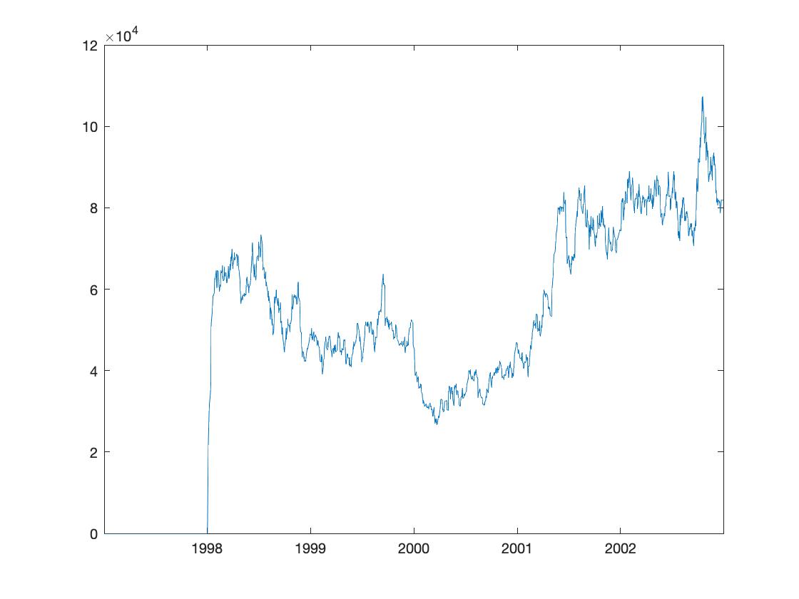
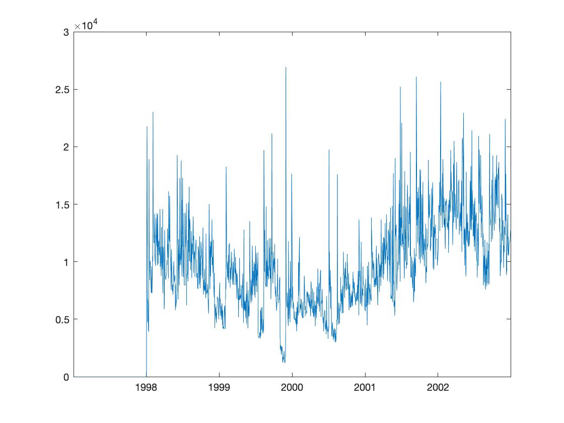
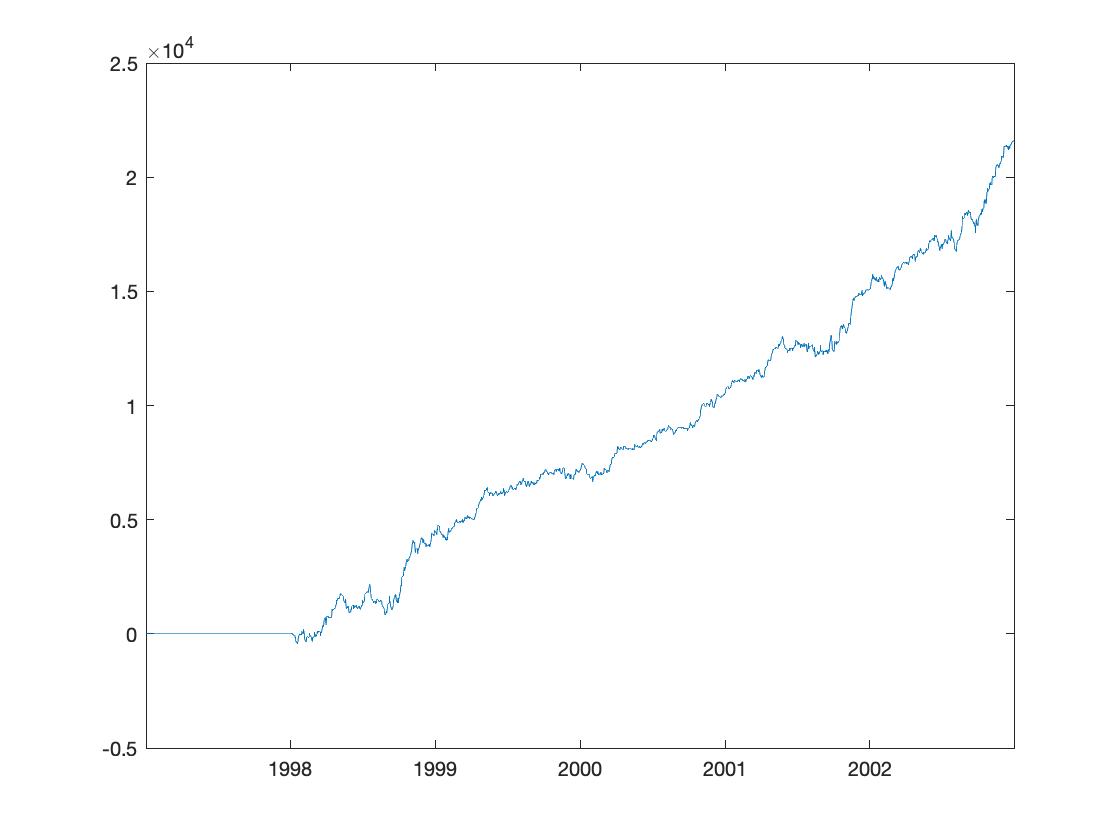
The backtesting result is recorded for each day in thousand dollars.

%% Backtest

booksize = sum(abs(back_weight), 2, 'omitnan');
tradesize = sum(abs(trade), 2, 'omitnan');

figure(1);
plot(dates, booksize);

figure(2);
plot(dates, tradesize);

figure(3);
pnl = cumsum(daily_pnl);
plot(dates, pnl);

Book Size
Trade Size
Profit & Loss

Performance Gauge

I calculated the Sharpe ratio, the maximum drawdown and the deepest drawdown for the performance of the portfolio. The Sharpe ratio is recorded as 2.640 for the long-short portfolio. And the longest drawdown is 29 days with $1.336M depth.

%% Performance
rf = 0;
excess_return = daily_pnl ./ booksize;

% sharpe ratio
sharpe = mean(excess_return, 'omitnan')*sqrt(252)/std(excess_return, 'omitnan');


for i=1:length(pnl)
    dd(i) = max(pnl(1:i)) - pnl(i);
end

% calculate maximum drawdown statistics
MDD = max(dd);
MDDe = find(dd==MDD);
MDDs = find(abs(pnl(MDDe)+ MDD - pnl) < 0.000001);

longest_dd = MDDe - MDDs;
deepest_dd = MDD;

Variable	Dimension	Definition
\(\mathbf{x}\)	\(n \times 1\)	desired portfolio weights
\(\mathbf{w}\)	\(n \times 1\)	initial portfolio weights
\(\boldsymbol{\Sigma}\)	\(n \times n\)	covariance matrix of stock returns
\(\boldsymbol{\alpha}\)	\(n \times 1\)	aggregate alphas
\(\boldsymbol{\beta}\)	\(n \times 1\)	historical betas
\(\boldsymbol{\tau}\)	\(n \times 1\)	transaction costs